《DEEP LEARNING with Python》第七章 深入了解 Keras
第七章 深入了解 Keras
A deep dive on Keras
运行代码
本章内容
- 创建 Keras 模型的不同方法:
Sequential类、函数式 API 和模型子类化 - 如何使用 Keras 内置的训练和评估循环,包括如何使用自定义指标和自定义损失函数。
- 使用 Keras 回调函数进一步自定义训练过程
- 使用 TensorBoard 来监控您的训练和评估指标随时间的变化
- 如何从零开始编写自己的训练和评估循环
你已经开始积累一些使用 Keras 的经验了。你熟悉Sequential模型、Dense层以及用于训练、评估和推理的内置 API——train、evaluate、compile()``fit()catch``evaluate()和 catch predict()。你甚至在第 3 章中学习了如何继承 Training 类 Layer来创建自定义层,以及如何使用 TensorFlow、JAX 和 PyTorch 中的梯度 API 来实现逐步训练循环。
在接下来的章节中,我们将深入探讨计算机视觉、时间序列预测、自然语言处理和生成式深度学习(computer vision, timeseries forecasting, natural language processing, and generative deep learning)。这些复杂的应用需要的远不止Sequential架构和默认fit()循环。所以,首先让我们把你培养成 Keras 专家!在本章中,你将全面了解使用 Keras API 的关键方法:你需要掌握的所有内容,足以应对接下来遇到的各种高级深度学习用例。
一系列工作流程
A spectrum of workflows
Keras API 的设计遵循 渐进式复杂性披露(progressive disclosure of complexity)原则:既要让用户轻松上手,又要能够处理高复杂度的用例,每一步只需循序渐进地学习。简单的用例应该简单易懂,而任意高级的工作流程也应该可行:无论你想做的事情多么小众或复杂,都应该有一条清晰的路径,这条路径建立在你从更简单的工作流程中学到的各种知识之上。这意味着你可以从新手成长为专家,并且仍然使用相同的工具——只是方式有所不同。
因此,使用 Keras 并没有唯一的“正确”方法。相反,Keras 提供了一系列工作流程,从非常简单到非常灵活。构建 Keras 模型的方法有很多种,训练模型的方法也各不相同,以满足不同的需求。
例如,构建模型的方法有很多种,训练模型的方法也多种多样,每种方法都代表着可用性和灵活性之间的一种权衡。你可以像使用 scikit-learn 一样使用 Keras——只需调用函数fit(),让框架自动完成所有工作——也可以像使用 NumPy 一样使用它——完全掌控每一个细节。
个人注:Scikit-learn(简称
sklearn)是 Python 中最流行、功能最强大的开源机器学习库之一。它建立在 NumPy、SciPy 和 Matplotlib 之上,为各种机器学习任务提供了简单、高效且一致的工具。
- 易用性:它拥有非常统一的 API 设计(所有的模型都使用
.fit()来训练,用.predict()来预测),学习曲线非常平缓。- 文档极其详尽:官方文档不仅包含 API 使用说明,还附带了大量的数学原理背景和精美的图表。
- 工业级性能:虽然它是用 Python 编写的,但底层核心计算任务通过 Cython、C 或 C++ 进行了优化,运行速度非常快。
- 活跃的社区:由于其广泛的用户基础,你在遇到问题时几乎总能快速找到解决方案。
虽然 Scikit-learn 非常强大,但它主要聚焦于传统机器学习(基于统计学的算法)。
- 如果你要处理结构化数据(如表格数据、Excel 数据),Scikit-learn 是首选。
- 如果你要处理非结构化数据(如超大规模的图像、长文本或语音信号),通常会转向专门的深度学习框架(如 TensorFlow, PyTorch, 或 JAX)。
由于所有这些工作流都基于共享的 API(例如 java.util.java``Layer和 java.util.java ),Model因此任何工作流中的组件都可以在任何其他工作流中使用:它们可以相互通信。这意味着,您现在入门所学的一切,在您成为专家之后仍然适用。您可以轻松上手,然后逐步深入到需要从头编写更多逻辑的工作流中。从学生到研究员,或者从数据科学家到深度学习工程师,您无需切换到完全不同的框架。
这种理念与 Python 本身的理念不谋而合!有些语言只提供一种编写程序的方式——例如面向对象编程或函数式编程。而 Python 则是一种多范式语言:它提供了一系列可能的编程模式,而且这些模式都能很好地协同工作。这使得 Python 适用于各种截然不同的应用场景:系统管理、数据科学、机器学习工程、Web 开发,甚至仅仅是学习编程。同样地,你可以把 Keras 看作是深度学习领域的 Python:一种用户友好的深度学习语言,为不同的用户群体提供了多种工作流程。
构建 Keras 模型的不同方法
Different ways to build Keras models
Keras 中用于构建模型的 API 有三种,如图 7.1 所示:
- 顺序模型是最容易上手的 API——它本质上就是一个 Python 列表。因此,它仅限于简单的层堆叠结构。
- 函数式 API专注于类似图的模型架构。它在易用性和灵活性之间取得了很好的平衡,因此,它是最常用的模型构建 API。
- 模型子类化是一种底层选项,需要您从头开始编写所有代码。如果您想要完全掌控每个细节,这非常理想。但是,您将无法使用许多 Keras 内置功能,并且更容易出错。
- The Sequential model is the most approachable API — it’s basically a Python list. As such, it’s limited to simple stacks of layers.
- The Functional API, which focuses on graph-like model architectures. It represents a nice mid-point between usability and flexibility, and as such, it’s the most commonly used model-building API.
- Model subclassing, a low-level option where you write everything yourself from scratch. This is ideal if you want full control over every little thing. However, you won’t get access to many built-in Keras features, and you will be more at risk of making mistakes.
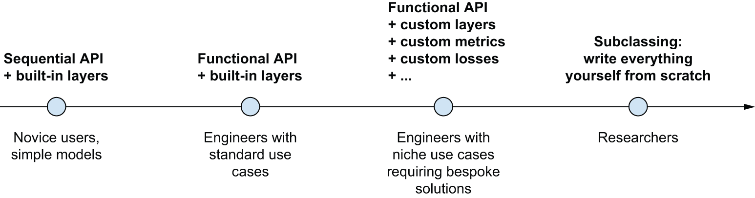 图 7.1:模型构建复杂性的逐步揭示
序列模型
The Sequential model
构建 Keras 模型的最简单方法就是Sequential你已经了解的模型。
1 | import keras |
清单 7.1:Sequential该类
请注意,可以通过该add() 方法逐步构建相同的模型,类似于append()Python 列表的方法。
1 | model = keras.Sequential() |
清单 7.2:逐步构建Sequential模型
在第三章中,你已经看到,层只有在第一次被调用时才会构建(也就是创建它们的权重)。这是因为层权重的形状取决于其输入的形状:在输入形状确定之前,它们无法被创建。
因此,之前的模型只有在你实际调用它处理一些数据,或者使用输入形状Sequential调用它的方法时,才具有权重。build()
1 | >>> # At that point, the model isn't built yet. |
清单 7.3:尚未建造的模型没有重量。
1 | >>> # Builds the model. Now the model will expect samples of shape |
清单 7.4:首次调用模型进行构建
模型构建完成后,可以通过该summary() 方法显示其内容,这对于调试非常方便。
1 | >>> model.summary() |
清单 7.5:汇总方法
如您所见,您的模型恰好被命名为 <model_name> sequential_1。实际上,在 Keras 中您可以为所有内容命名——每个模型、每一层。
1 | >>> model = keras.Sequential(name="my_example_model") |
清单 7.6name :使用参数 命名模型和层
在逐步构建Sequential模型时,每添加一层后,打印出当前模型的概要信息会很有用。但是,在模型构建完成之前,你无法打印概要信息!实际上,有一种方法可以让Sequential模型动态构建:只需预先声明模型输入的结构即可。你可以通过Input类来实现这一点。
1 | model = keras.Sequential() |
清单 7.7:预先指定模型的输入形状
现在你可以用它summary()来观察随着你添加更多层,模型的输出形状是如何变化的:
1 | >>> model.summary() |
对于以复杂方式转换输入的层(例如您将在第 8 章中学到的卷积层),这是一个相当常见的调试工作流程。
函数式 API
The Functional API
该Sequential模型易于使用,但适用范围极其有限:它只能表示具有单个输入和单个输出的模型,并且需要按顺序逐层应用。然而,在实践中,我们经常会遇到具有多个输入(例如,图像及其元数据)、多个输出(想要预测的不同数据特征)或非线性拓扑结构的模型。
The Sequential model is easy to use, but its applicability is extremely limited: it can only express models with a single input and a single output, applying one layer after the other in a sequential fashion. In practice, it’s pretty common to encounter models with multiple inputs (say, an image and its metadata), multiple outputs (different things you want to predict about the data), or a nonlinear topology.
在这种情况下,您可以使用函数式 API 构建模型。大多数 Keras 模型在实际应用中都会使用这种方式。它既有趣又强大——感觉就像在玩乐高积木一样。
一个简单的例子
A simple example
我们先从简单的例子开始:上一节中使用的两层协议栈。它的函数式 API 版本如下所示。
1 | inputs = keras.Input(shape=(3,), name="my_input") |
清单 7.8Dense :一个简单的两层 函数式模型
让我们一步一步来。首先,我们声明了一个输入对象Input (请注意,您也可以像其他所有对象一样,为这些输入对象命名):
1 | inputs = keras.Input(shape=(3,), name="my_input") |
该inputs对象包含有关形状以及dtype模型将要处理的数据的信息:
1 | >>> # The model will process batches where each sample has shape (3,). |
我们将这样的对象称为符号张量。它不包含任何实际数据,而是编码了模型在使用时将要看到的实际数据张量的规范。它代表未来的数据张量。
We call such an object a symbolic tensor. It doesn’t contain any actual data, but it encodes the specifications of the actual tensors of data that the model will see when you use it. It stands for future tensors of data.
接下来,我们创建了一个图层并将其应用于输入:
1 | features = layers.Dense(64, activation="relu")(inputs) |
所有 Keras 层既可以对真实数据张量调用,也可以对这些符号张量调用。在后一种情况下,它们会返回一个新的符号张量,其中包含更新后的形状和数据类型信息:
1 | >>> features.shape |
获得最终输出后,我们在Model构造函数中指定模型的输入和输出,从而实例化该模型:
1 | outputs = layers.Dense(10, activation="softmax")(features) |
以下是我们模型的概要:
1 | >>> model.summary() |
多输入多输出模型
Multi-input, multi-output models
与这个玩具模型不同,大多数深度学习模型看起来不像列表,而更像图。例如,它们可能具有多个输入或多个输出。函数式 API 的优势正体现在这类模型上。
假设您正在构建一个系统,用于按优先级对客户支持工单进行排序,并将其路由到相应的部门。您的模型有三个输入:
- 票号(文本输入)
- 票面文本(文本输入)
- 用户添加的任何标签(分类输入,此处假设为多热编码)
我们可以将文本输入编码为大小为 1 和 0 的数组vocabulary_size (有关文本编码技术的详细信息,请参阅第 14 章)。
您的模型也有两个输出:
- 工单优先级得分,介于 0 和 1 之间的标量(sigmoid 输出)
- 应该处理此工单的部门(对部门集合进行 softmax 处理)
使用函数式 API,只需几行代码即可构建此模型。
1 | vocabulary_size = 10000 |
清单 7.9:多输入多输出功能模型
函数式 API 是一种简单、类似乐高积木但又非常灵活的方式来定义像这样的任意层图。
训练多输入多输出模型
Training a multi-input, multi-output model
你可以用与训练普通模型类似的方式训练你的模型Sequential,即通过调用函数并传入fit()输入和输出数据列表。这些数据列表的顺序应该与你传递给构造函数的输入顺序一致Model()。
1 | import numpy as np |
清单 7.10:通过提供输入数组和目标数组列表来训练模型
如果您不想依赖输入顺序(例如,因为您有很多输入或输出),您还可以使用您给对象Input和输出层赋予的名称,并通过字典传递数据。
1 | model.compile( |
清单 7.11:通过提供输入和目标数组的字典来训练模型
个人注:
model.fit里的验证(留出法)当你写
model.fit(x, y, validation_split=0.2)时:
- 数据分配:它在训练开始前,固定切下最后 20% 的数据作为验证集。
- 过程:
- 第一轮(Epoch 1):用前 80% 练,用固定的后 20% 验。
- 第二轮(Epoch 2):还是用前 80% 练,用固定的后 20% 验。
- ...以此类推。
- 本质:这 20% 的数据从头到尾都没参与过“举一反三”的训练,它们自始至终只是观众。
- K 折交叉验证(K-Fold)
K 折交叉验证是一个更高级别的循环,它不是在一个
fit里完成的,而是要跑 K 个独立的fit。
- 数据分配:数据被分成 K 份(比如 5 份)。
- 过程:
- 第一次 fit:用第 1,2,3,4 份练,用第 5 份验。得到一个模型性能。
- 第二次 fit:清空模型权重,重新开始。用第 1,2,3,5 份练,用第 4 份验。得到另一个性能。
- ...重复 5 次。
- 本质:每一份数据都既当过老师(训练集),又当过考官(验证集)。
model.evaluate():评估模式这是对模型进行“考试”的过程。
动作:模型读取测试数据,进行前向传播得到预测结果,并计算损失和指标(如准确率)。但它不会执行反向传播,也不会改变模型的任何参数。
最终检查:训练过程中的验证集表现可能被开发者用来调整超参数(如学习率),这可能导致模型对验证集产生“间接偏见”。
evaluate通常用于最后的、完全独立的测试集,以获得最公正的泛化能力评估。部署前验证:在保存模型并重新加载后,可以使用
evaluate快速确认模型在特定数据集上的性能是否符合预期。 如果你只想获得预测结果而不需要计算损失或指标,你应该使用model.predict(),它只返回预测的输出值。
函数式 API 的强大功能:访问层连接
The power of the Functional api: Access to layer connectivity
函数式模型是一种显式的图数据结构。这使得我们可以检查各层之间的连接方式,并将先前的图节点 (即各层的输出)重用于新模型中。它也很好地契合了大多数研究人员在思考深度神经网络时所使用的“心智模型”:一个由各层构成的图。
A Functional model is an explicit graph data structure. This makes it possible to inspect how layers are connected and reuse previous graph nodes (which are layer outputs) as part of new models. It also nicely fits the “mental model” that most researchers use when thinking about a deep neural network: a graph of layers.
这实现了两个重要的应用场景:模型可视化和特征提取。让我们一起来看看。
绘制层连通性
Plotting layer connectivity
让我们将刚才定义的模型的连接性(模型的拓扑结构)可视化。您可以使用工具将函数模型绘制成图plot_model(),如图 7.2 所示:
1 | keras.utils.plot_model(model, "ticket_classifier.png") |
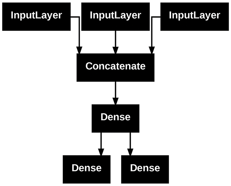 图 7.2
图 7.2plot_model() :由我们的票务分类模型 生成的图表
您可以在此图中添加模型中每一层的输入和输出形状,以及层名称(而不仅仅是层类型),这在调试期间会很有帮助(图 7.3):
1 | keras.utils.plot_model( |
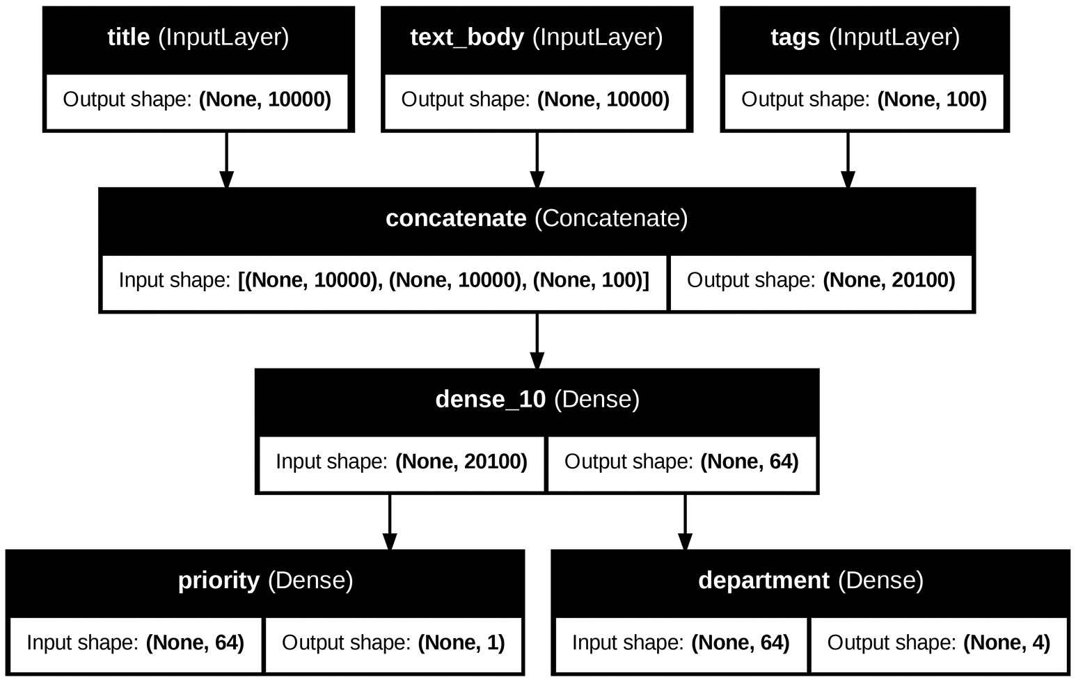 图 7.3:添加了形状信息的模型图
张None量形状中的 表示批次大小:此模型允许任意大小的批次。
基于函数模型的特征提取
Feature extraction with a Functional model
访问层连接还意味着您可以检查和重用图中的各个节点(层调用)。模型属性model.layers 提供构成模型的层列表,您可以对每一层进行layer.input查询layer.output。
1 | >>> model.layers |
清单 7.12:检索函数模型中某一层的输入或输出
这样就可以进行特征提取:创建能够重用另一个模型中的中间特征的模型。
假设你想在我们之前定义的模型中添加另一个输出——你还想预测某个问题工单的解决时间,也就是一个难度等级。你可以通过一个分类层来实现,该分类层分为三个类别:“快速”、“中等”和“困难”。你不需要从头开始重新创建和训练模型!你可以直接从之前模型的中间特征入手,因为你已经可以访问这些特征。
1 | # layers[4] is our intermediate Dense layer. |
清单 7.13:通过重用中间层输出创建新模型
让我们绘制出新模型,如图 7.4 所示:
1 | keras.utils.plot_model( |
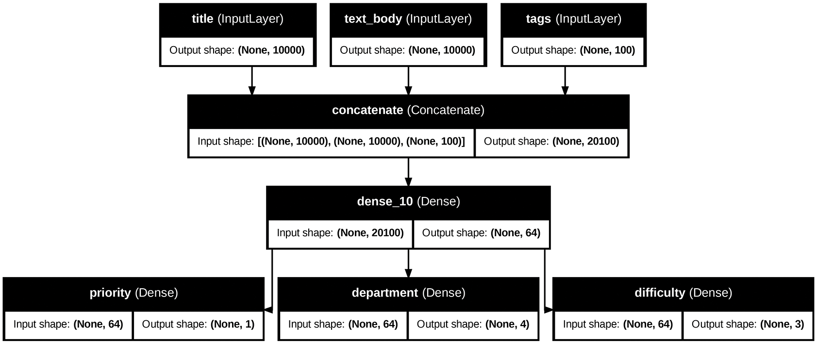 图 7.4:我们新模型的示意图
对 Model 类进行子类化
Subclassing the Model class
你需要了解的最后一种模型构建模式是最高级的: Model子类化。你已经在第 3 章学习了如何通过子类化Layer来创建自定义层。子类化Model与之非常相似:
- 在
__init__方法中,定义模型将使用的层。 - 在该
call方法中,定义模型的前向传播,重用先前创建的层。 - 实例化你的子类,并调用它来获取数据,从而创建其权重。
将之前的示例重写为子类模型
Rewriting our previous example as a subclassed model
让我们来看一个简单的例子:我们将使用Model子类重新实现客户支持工单管理模型。
1 | class CustomerTicketModel(keras.Model): |
清单 7.14:一个简单的子类化模型
定义好模型后,就可以实例化它了。请注意,它只会在第一次使用某些数据调用它时创建权重——Layer这与子类非常相似:
1 | model = CustomerTicketModel(num_departments=4) |
到目前为止,一切看起来都与Layer子类化非常相似,这是你在第 3 章已经接触过的工作流程。那么,Layer子类和Model子类之间有什么区别呢?很简单:层是用来创建模型的基本构建块,而模型是你实际训练、导出用于推理等的顶层对象。简而言之,模型Model有 map fit()、 map``evaluate()和 predict()map 方法。层没有。除此之外,这两个类几乎完全相同(另一个区别是你可以将模型保存到磁盘上的文件中——我们将在后面的章节中介绍这一点)。
您可以Model像编译序列模型或函数模型一样编译和训练子类:
1 | model.compile( |
子Model类化工作流程是构建模型最灵活的方式:它使您能够构建无法用层级有向无环图表示的模型——例如,想象一下这样一个模型:方法call()在循环中使用层级for,甚至递归调用它们。一切皆有可能——一切由您掌控。
注意:哪些子类模型不支持
Beware: What subclassed models don’t support
这种自由是有代价的:使用子类模型,你需要负责更多模型逻辑,这意味着潜在的错误范围更大。因此,你需要进行更多的调试工作。你是在开发一个新的 Python 对象,而不是简单地拼搭乐高积木。
函数式模型和子类模型本质上也截然不同:函数式模型是一种显式的数据结构——一个层级图,你可以查看、检查和修改它。而子类模型则是一段字节码——一个包含call()原始代码方法的 Python 类。这正是子类化工作流程灵活性的来源——你可以编写任何你想要的功能——但同时也引入了新的限制。
例如,由于层之间的连接方式隐藏在方法体内部call(),因此您无法访问该信息。调用该方法summary()不会显示层连接,您也无法通过该方法绘制模型拓扑plot_model()。同样,如果您有一个子类化的模型,则无法访问层图的节点来进行特征提取——因为根本没有层图。模型实例化后,其前向传播过程就变成了一个完全的黑盒。
混合搭配不同的组件
Mixing and matching different components
至关重要的是,选择这些模式中的任何一种——Sequential模型、函数式 API 或Model子类化——都不会限制您使用其他模式。Keras API 中的所有模型都可以彼此无缝互操作,无论是序列模型、函数式模型还是从头编写的子类化模型。它们都属于同一工作流程范畴。例如,您可以在函数式模型中使用子类化的层或模型。
1 | class Classifier(keras.Model): |
清单 7.15:创建包含子类化模型的功能模型
反之,您也可以将函数模型用作子类层或模型的一部分。
1 | inputs = keras.Input(shape=(64,)) |
清单 7.16:创建包含函数模型的子类模型
记住:做事要用对工具
Remember: Use the right tool for the job
您已经了解了构建 Keras 模型的各种工作流程,从最简单的工作流程——Sequential直接创建模型——到最复杂的工作流程——模型子类化。那么,何时应该使用哪一种呢?每种工作流程都有其优缺点——请根据具体情况选择最合适的。
总的来说,函数式 API 在易用性和灵活性之间取得了相当不错的平衡。它还允许您直接访问图层连接,这对于模型绘图或特征提取等用例非常强大。如果您可以使用函数式 API(也就是说,如果您的模型可以表示为图层的有向无环图),我们建议您使用它而不是模型子类化。
接下来,本书中的所有示例都将使用函数式 API——原因很简单,因为我们使用的所有模型都可以表示为层图。不过,我们会频繁使用子类化层。总的来说,使用包含子类化层的函数式模型可以兼顾两者的优势:既能保持高度的开发灵活性,又能保留函数式 API 的优点。
利用内置的训练和评估循环
Using built-in training and evaluation loops
逐步揭示复杂性的原则——即逐步提供从极其简单到任意灵活的一系列工作流程——同样适用于模型训练。Keras 提供了不同的模型训练工作流程——既可以像调用 fit()现有数据那样简单,也可以像从头开始编写新的训练算法那样复杂。
您应该已经熟悉了compile(),,,工作流程fit()。 提醒一下,它看起来像下面这个列表evaluate()。predict()
个人注:在 Keras 的模型生命周期中,
model.compile()和model.fit()分别代表了两个完全不同的阶段:配置阶段和执行阶段。简单来说:
compile是告诉模型“规则是什么”,而fit是让模型“开始练习”。
model.compile():配置规则(设置“考试大纲”)在这一步,模型并没有接触到你的实际数据。你是在定义模型在训练时应该如何优化自己。
- 主要任务:
- 选择优化器 (Optimizer):决定模型如何更新权重(例如:
Adam,SGD)。- 定义损失函数 (Loss Function):决定模型如何计算预测值与真实值之间的差距(例如:
categorical_crossentropy,mse)。- 选择评估指标 (Metrics):决定我们在训练过程中关注什么(例如:
accuracy)。
1 | from keras.datasets import mnist |
清单 7.17:标准工作流程:compile(),,,fit()``evaluate()``predict()
您可以通过以下几种方式自定义此简单工作流程:
- 通过提供您自己的自定义指标
- 通过向该方法传递回调函数
fit(),可以在训练期间的特定时间点安排要执行的操作。
我们来看一下这些。
编写自己的指标
Writing your own metrics
指标是衡量模型性能的关键——尤其对于衡量模型在训练数据和测试数据上的性能差异而言。分类和回归常用的指标已经包含在内置keras.metrics模块中——大多数情况下,您都会使用这些内置指标。但如果您要进行一些非常规操作,则需要能够编写自己的指标。这很简单!
Keras 指标是keras.metrics.Metric层的一个子类。与层类似,指标也拥有存储在 Keras 变量中的内部状态。但与层不同的是,这些变量不会通过反向传播进行更新,因此您需要自行编写状态更新逻辑——这在update_state()方法中实现。例如,以下是一个简单的自定义指标,用于测量均方根误差 (RMSE)。
1 | from keras import ops |
清单 7.18Metric :通过继承类 来实现自定义指标
您可以使用该result()方法返回指标的当前值:
1 | def result(self): |
同时,您还需要提供一种无需重新实例化即可重置指标状态的方法——这使得相同的指标对象可以在不同的训练周期或训练和评估过程中使用。您可以在以下reset_state()方法中实现这一点:
1 | def reset_state(self): |
自定义指标的使用方法与内置指标相同。让我们来测试一下我们自己的指标:
1 | model = get_mnist_model() |
现在您可以看到fit()进度条显示模型的均方根误差 (RMSE)。
使用回调函数
Using callbacks
使用 Keras 对大型数据集进行数十个 epoch 的训练,model.fit() 有点像放飞纸飞机:除了最初的弹射之外,你无法控制它的轨迹或落点。为了避免糟糕的结果(从而避免浪费纸飞机),更明智的做法不是使用纸飞机,而是使用能够感知环境、将数据发送回操作员并根据当前状态自动做出转向决策的无人机。Keras回调API 可以帮助你将对 Keras 的调用model.fit()从纸飞机转变为能够自我评估并动态采取行动的智能自主无人机。
回调函数是一个对象(实现了特定方法的类实例),它在模型调用时被传递给模型fit(),并在训练过程中被模型在不同的阶段调用。它可以访问所有关于模型状态和性能的可用数据,并且可以执行以下操作:中断训练、保存模型、加载不同的权重集,或以其他方式改变模型的状态。
以下是一些使用回调函数的示例:
- 模型检查点 ——在训练过程中不同阶段保存模型的当前状态。
- 提前停止 ——当验证损失不再改善时中断训练(当然,还要保存训练期间获得的最佳模型)。
- 在训练过程中动态调整某些参数的值 ——例如优化器的学习率。
- 在训练过程中记录训练和验证指标,或者在模型学习到的表示更新时将其可视化 ——
fit()您熟悉的进度条实际上是一个回调! - Model checkpointing — Saving the current state of the model at different points during training.
- Early stopping — Interrupting training when the validation loss is no longer improving (and of course, saving the best model obtained during training).
- Dynamically adjusting the value of certain parameters during training — Such as the learning rate of the optimizer.
- Logging training and validation metrics during training, or visualizing the representations learned by the model as they’re updated — The
fit()progress bar that you’re familiar with is in fact a callback!
该keras.callbacks模块包含许多内置回调函数(以下并非完整列表):
1 | keras.callbacks.ModelCheckpoint |
让我们回顾其中两个例子,以便您了解如何使用它们: EarlyStopping和ModelCheckpoint。
EarlyStopping 和 ModelCheckpoint 回调
The EarlyStopping and ModelCheckpoint callbacks
在训练模型时,有很多事情是无法预先预测的。特别是,你无法确定需要多少轮训练才能达到最优的验证损失。我们目前的示例采用的策略是:先训练足够多的轮数,直到模型开始过拟合,然后用第一次训练的结果来确定最优轮数,最后再用这个最优轮数从头开始进行新的训练。当然,这种方法很浪费资源。更好的方法是,当验证损失不再改善时就停止训练。这可以通过EarlyStopping回调函数来实现。
当被监控的目标指标在固定的训练轮数内停止提升时,回调函数EarlyStopping会中断训练。例如,该回调函数允许您在模型开始过拟合时立即中断训练,从而避免需要重新训练模型以减少训练轮数。该回调函数通常与 save_model 函数结合使用ModelCheckpoint,后者允许您在训练过程中持续保存模型(并且可以选择仅保存当前最佳模型:即在每个训练轮结束时性能最佳的模型版本)。
1 | # Callbacks are passed to the model via the callbacks argument in |
清单 7.19 :在方法 callbacks中使用参数fit()
请注意,训练完成后您也可以随时手动保存模型——只需调用即可model.save("my_checkpoint_path.keras")。要重新加载已保存的模型,请使用。
1 | model = keras.models.load_model("checkpoint_path.keras") |
编写自己的回调函数
Writing your own callbacks
如果在训练过程中需要执行内置回调函数未涵盖的特定操作,您可以编写自己的回调函数。回调函数通过继承类来实现keras.callbacks.Callback。您可以实现以下任意数量的透明命名方法,这些方法会在训练过程中的不同阶段被调用:
1 | # Called at the start of every epoch |
这些方法都需要一个参数,该参数是一个字典,其中包含有关前一个批次、轮次或训练运行的logs信息:训练和验证指标等等。and 方法还接受轮次或批次索引作为第一个参数(一个整数)。on_epoch_*``on_batch_*
这里有一个简单的回调示例,它会在训练期间保存每个批次的损失值列表,并在每个 epoch 结束时绘制这些值。
1 | from matplotlib import pyplot as plt |
清单 7.20Callback :通过继承类 来创建自定义回调
我们来试驾一下:
1 | model = get_mnist_model() |
我们得到的图表类似于图 7.5。
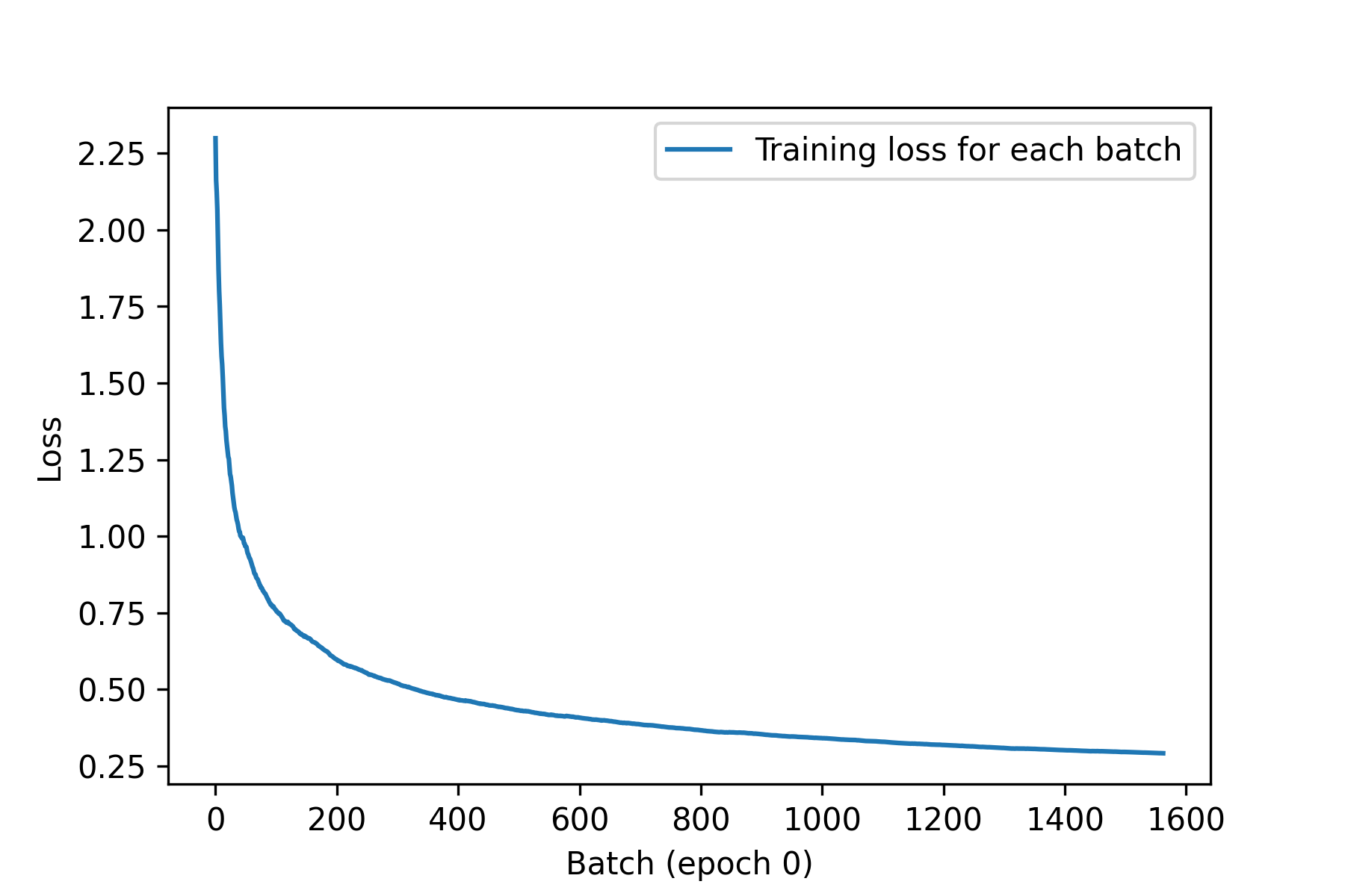 图 7.5:我们自定义历史绘图回调函数的输出
使用 TensorBoard 进行监控和可视化
Monitoring and visualization with TensorBoard
要做好研究或开发优秀的模型,你需要在实验过程中获得关于模型内部运行情况的丰富且频繁的反馈。这正是运行实验的目的:获取模型性能的尽可能多的信息。取得进展是一个迭代过程,一个循环:你从一个想法开始,将其转化为一个实验,尝试验证或推翻你的想法。你运行这个实验并处理它生成的信息,如图 7.6 所示。这会激发你的下一个想法。你运行的循环次数越多,你的想法就越完善、越强大。Keras 可以帮助你以最短的时间从想法到实验,而快速的 GPU 可以帮助你以最快的速度从实验到结果。但是如何处理实验结果呢?这就是 TensorBoard 的用武之地。
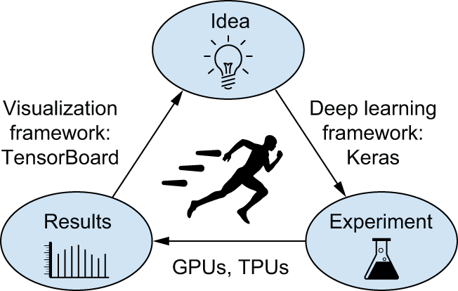 图 7.6:进度循环
TensorBoard 是一款基于浏览器的应用程序,可以本地运行。它是监控模型训练过程中所有运行情况的最佳方式。使用 TensorBoard,您可以:
- 在训练过程中直观地监控各项指标
- 可视化您的模型架构
- 可视化激活值和梯度直方图
- 探索 3D 嵌入
- Visually monitor metrics during training
- Visualize your model architecture
- Visualize histograms of activations and gradients
- Explore embeddings in 3D
如果您监控的信息不仅仅是模型的最终损失,您就可以更清楚地了解模型的功能和不足之处,从而更快地取得进展。
将 TensorBoard 与 Keras 模型和fit()方法结合使用的最简单方法是 keras.callbacks.TensorBoard使用回调函数。最简单的情况下,只需指定回调函数将日志写入的位置即可:
1 | model = get_mnist_model() |
模型开始运行后,会将日志写入目标位置。如果您在本地计算机上运行 Python 脚本,则可以使用以下命令启动本地 TensorBoard 服务器(请注意,tensorboard如果您已通过 TensorFlow 安装,则可执行文件应该已经可用pip;否则,您可以手动通过 TensorBoard 安装pip install tensorboard):
1 | tensorboard --logdir /full_path_to_your_log_dir |
然后,您可以导航到命令返回的 URL 以访问 TensorBoard 界面。
如果您在 Colab notebook 中运行脚本,则可以使用以下命令在 notebook 中运行嵌入式 TensorBoard 实例:
1 | %load_ext tensorboard |
在 TensorBoard 界面中,您可以监控训练和评估指标的实时图表,如图 7.7 所示。
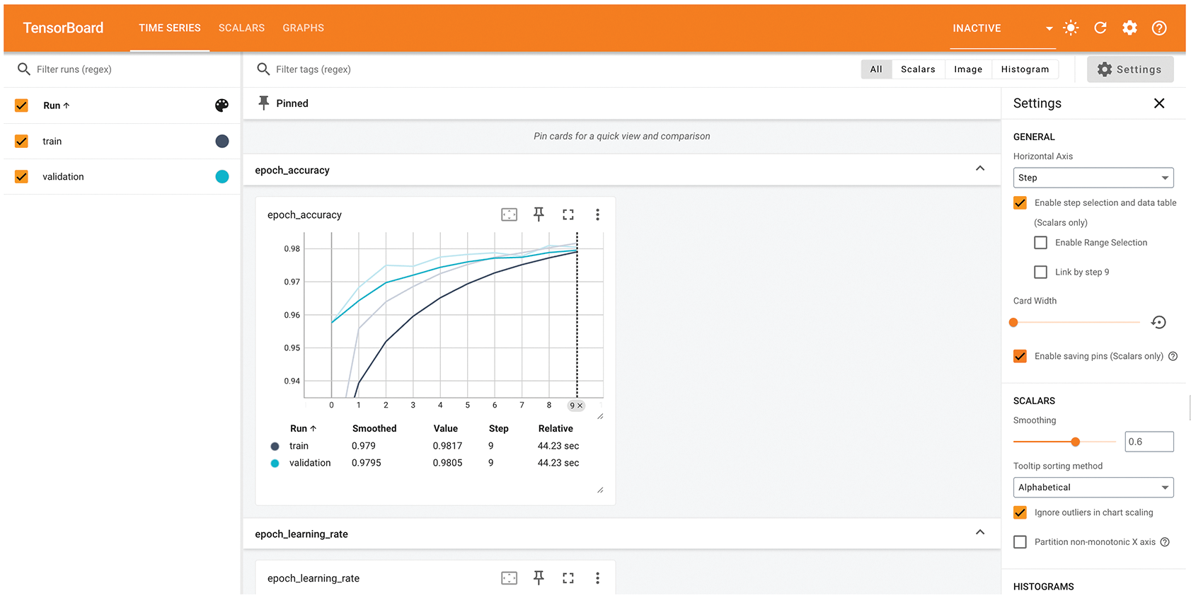 图 7.7:TensorBoard 可用于轻松监控训练和评估指标。
编写自己的培训和评估流程
Writing your own training and evaluation loops
该fit()工作流程在易用性和灵活性之间取得了很好的平衡,大部分时间您都会用到它。但是,它并非旨在支持深度学习研究人员可能想要做的所有事情——即使使用自定义指标、自定义损失函数和自定义回调函数。
毕竟,内置fit()工作流程仅专注于监督学习:在这种设置下,输入数据关联着已知的目标(也称为标签或标注),并且损失是根据这些目标和模型的预测结果计算得出的。然而,并非所有形式的机器学习都属于这一范畴。还有一些设置中不存在明确的目标,例如生成式学习(我们将在第 16 章介绍)、 自监督学习(目标从输入中获取)或 强化学习(学习由偶尔的“奖励”驱动——很像训练狗)。即使您进行的是常规的监督学习,作为研究人员,您可能也希望添加一些新颖的功能,而这些功能需要底层灵活性。
After all, the built-in fit() workflow is solely focused on supervised learning: a setup where there are known targets (also called labels or annotations) associated with your input data and where you compute your loss as a function of these targets and the model’s predictions. However, not every form of machine learning falls into this category. There are other setups where no explicit targets are present, such as generative learning (which we will introduce in chapter 16), self-supervised learning (where targets are obtained from the inputs), or reinforcement learning (where learning is driven by occasional “rewards”—much like training a dog). And even if you’re doing regular supervised learning, as a researcher, you may want to add some novel bells and whistles that require low-level flexibility.
当您发现内置功能fit()不足以满足需求时,就需要编写自定义训练逻辑。您已经在第 2 章和第 3 章中看到了底层训练循环的简单示例。作为提醒,典型的训练循环内容如下所示:
- 运行“前向传播”(计算模型的输出)以获得当前批次数据的损失值。
- 获取损失函数相对于模型权重的梯度。
- 更新模型的权重,以降低当前数据批次的损失值。
这些步骤会重复进行,直到处理完所有需要的批次。这基本上就是fit()底层实现的原理。在本节中,你将学习如何fit()从头开始重新实现,这将为你编写任何你想要的训练算法提供所需的全部知识。
让我们来详细了解一下。在接下来的几节中,你将逐步学习如何使用 TensorFlow、PyTorch 和 JAX 编写功能齐全的自定义训练循环。
训练与推理
Training vs. inference
在你目前看到的底层训练循环示例中,步骤 1(前向传播)是通过 map 完成的predictions = model(inputs),而步骤 2(检索梯度带计算出的梯度)是通过后端特定的 API 完成的,例如 map。
gradients = tape.gradient(loss, model.weights)在 TensorFlow 中loss.backward()在 PyTorch 中jax.value_and_grad()在 JAX
一般来说,其实有两个细微之处需要考虑。
某些 Keras 层(例如 map层)在训练和推理 (用于生成预测)期间Dropout的行为有所不同。这类层在其 map 方法中公开了一个布尔参数。调用 map会丢弃一些激活值,而调用 map 则不会执行任何操作。同样,函数式模型和序列模型也在 其 map 方法中公开了此参数。请记住, 在前向传播期间调用 Keras 模型时,必须传递此参数!因此,我们的前向传播过程将变为 map 。training``call()``dropout(inputs, training=True)``dropout(inputs, training=False)``training``call()``training=True``predictions = model(inputs, training=True)
此外,请注意,在检索模型权重梯度时,不应使用 ggradients model.weights,而应使用 ggradients model.trainable_weights。实际上,层和模型都有两种类型的权重:
- 可训练权重,旨在通过反向传播进行更新,以最小化模型的损失,例如
Dense层的核和偏置。 - 不可训练权重是指在前向传播过程中由拥有它们的层进行更新的权重。例如,如果您希望自定义层记录已处理的批次数量,则该信息将存储在不可训练权重中,并且在每个批次处理过程中,该层会将计数器加一。
在 Keras 内置层中,唯一具有不可训练权重的层是BatchNormalization第 9 章将要介绍的层。该BatchNormalization层需要不可训练的权重来跟踪有关通过它的数据的均值和标准差的信息,以便执行 特征归一化的在线近似(这是你在第 4 章和第 6 章中学到的概念)。
编写自定义训练步骤函数
Writing custom training step functions
考虑到这两个细节,监督学习的训练步骤最终可以用伪代码表示如下:
1 | def train_step(inputs, targets): |
这段代码是伪代码而不是实际代码,因为它包含一个虚构的函数get_gradients_of()。实际上,梯度的获取方式取决于你当前的后端——JAX、TensorFlow 或 PyTorch。
让我们运用第三章中学到的各个框架的知识,来实现这个train_step()函数的实际版本。我们先从 TensorFlow 和 PyTorch 开始,因为这两个框架相对来说比较容易上手,所以是很好的起点。最后我们会用到 JAX,它要复杂得多。
TensorFlow 训练步骤函数
A TensorFlow training step function
TensorFlow 允许你编写与我们的伪代码片段非常相似的代码。唯一的区别在于,你的前向传播应该在一个作用域内进行GradientTape 。然后,你可以使用该tape对象来检索梯度:
1 | import tensorflow as tf |
我们来运行一个步骤:
1 | batch_size = 32 |
很简单!接下来我们学习 PyTorch。
PyTorch 训练步骤函数
A PyTorch training step function
当您使用 PyTorch 后端时,您的所有 Keras 层和模型都会继承自 PyTorchtorch.nn.Module 类并公开原生ModuleAPI。因此,您的模型、其可训练权重和损失张量彼此感知,并通过以下三个方法进行交互:loss.backward()、weight.value.grad和model.zero_grad()。
回顾第三章的内容,你需要牢记的思维模式是这样的:
- 在每次前向传播过程中,PyTorch 都会构建一个一次性的计算图,用于跟踪刚刚发生的计算。
- 调用
.backward()此图中的任何给定标量节点(例如您的损失函数)都会从该节点开始反向运行该图,并自动填充tensor.grad所有相关张量(如果它们满足条件requires_grad=True)的属性,该属性包含输出节点相对于该张量的梯度。具体来说,它会填充grad可训练参数的属性。 - 要清除该属性的内容
tensor.grad,您应该tensor.grad = None对所有张量调用该函数。由于逐个对所有模型变量执行此操作会比较繁琐,因此您只需在模型级别通过clear()函数进行操作即可model.zero_grad()——该zero_grad()调用将传播到模型跟踪的所有变量。清除梯度至关重要,因为clear()函数的调用backward()是累加的:如果您不在每个步骤中清除梯度,梯度值将不断累积,训练将无法继续进行。
让我们按顺序执行这些步骤:
1 | import torch |
我们来运行一个步骤:
1 | batch_size = 32 |
这并不难!现在,我们继续学习 JAX。
JAX 训练步骤函数
A JAX training step function
就底层训练代码而言,由于 JAX 完全无状态的特性,它往往是三种后端中最复杂的。无状态特性使得 JAX 具有极高的性能和可扩展性,使其易于编译和自动性能优化。然而,编写无状态代码需要克服一些障碍。
由于梯度函数是通过元编程获得的,因此首先需要定义返回损失的函数。此外,该函数必须是无状态的,因此它需要接收所有将要使用的变量作为参数,并返回任何已更新变量的值。还记得那些在前向传播过程中可以被修改的不可训练权重吗?这些就是我们需要返回的变量。
为了更方便地使用 JAX 的无状态编程范式,Keras 模型提供了一个无状态的前向传递方法:getState()``stateless_call()方法。它的行为与 getState() 类似__call__,区别在于:
- 它除了接受模型的可训练权重和不可训练权重作为输入外,还接受
inputsand``training参数。 - 除了模型的输出之外,它还会返回模型的更新后的不可训练权重。
它的工作原理如下:
1 | outputs, non_trainable_weights = model.stateless_call( |
我们可以使用stateless_call()JAX 来实现我们的损失函数。由于该损失函数还会计算所有不可训练变量的更新,因此我们将其命名为compute_loss_and_updates():
1 | model = get_mnist_model() |
有了这个compute_loss_and_updates()函数之后,我们就可以把它传递给它jax.value_and_grad来进行梯度计算:
1 | import jax |
现在,这里有个小问题。and``jax.grad()和or 都jax.value_and_grad() 要求fn只返回标量值。我们的compute_loss_and_updates() 函数返回一个标量值作为第一个输出,但它也返回了不可训练权重的新值。还记得第三章学过的内容吗?解决方法是给or传递一个has_aux参数,像这样:grad()``value_and_grad()
1 | import jax |
使用方法如下:
1 | (loss, non_trainable_weights), gradients = grad_fn( |
好了,刚才讲了很多关于 JAX 的内容。但现在我们几乎拥有了构建 JAX 训练步骤所需的一切。我们只需要最后一块拼图optimizer.apply():
在第二章开头,当你用 TensorFlow 编写第一个基本训练步骤时,你编写了一个如下所示的更新步骤函数:
1 | learning_rate = 1e-3 |
这与优化器的工作方式相符keras.optimizers.SGD。然而,Keras API 中的其他优化器都比这复杂一些,它们会跟踪一些辅助变量来加速训练——特别是,大多数优化器都使用某种形式的动量,你在第二章中已经学过。这些额外的变量会在训练的每个步骤中更新,在 JAX 中,这意味着你需要一个无状态函数,该函数接受这些变量作为参数并返回它们的新值。
为了方便起见,Kerasstateless_apply()在所有优化器中都提供了该方法。其工作原理如下:
1 | trainable_variables, optimizer_variables = optimizer.stateless_apply( |
现在,我们已经掌握了足够的信息来构建一个完整的培训流程:
1 | optimizer = keras.optimizers.Adam() |
我们来运行一个步骤:
1 | batch_size = 32 |
虽然 JAX 的开发工作量肯定比 TensorFlow 和 PyTorch 要大一些,但它的速度和可扩展性优势足以弥补这一点。
接下来,我们来看自定义训练循环的另一个重要元素:指标。
指标的低级使用
Low-level usage of metrics
在底层训练循环中,你可能需要使用 Keras 指标(无论是自定义指标还是内置指标)。你已经了解了指标 API:只需update_state(y_true, y_pred)对每个目标和预测批次调用该 API,然后使用result()该 API 查询当前指标值即可。
1 | from keras import ops |
您可能还需要跟踪标量值的平均值,例如模型的损失。您可以通过以下keras.metrics.Mean指标来实现:
1 | values = ops.array([0, 1, 2, 3, 4]) |
metric.reset_state()记住,当你想要重置当前结果时(在训练周期开始时或评估开始时),可以使用此功能。
如果您使用的是 JAX,则 不能在无状态函数中使用类似 getState()``update_state()或 getState() 这样的状态修改方法。不过,您可以使用无状态指标 API,它类似于您之前了解的 getState()和 getState () 方法。以下是它的工作原理:reset()``model.stateless_call()``optimizer.stateless_apply()
1 | metric = keras.metrics.SparseCategoricalAccuracy() |
使用 fit() 函数和自定义训练循环
Using fit() with a custom training loop
在前面的章节中,我们完全从零开始编写自己的训练逻辑。这样做虽然提供了最大的灵活性,但最终会编写大量的代码,同时还会错过许多便捷的功能fit(),例如回调、性能优化或对分布式训练的内置支持。
如果你需要自定义训练算法,但又想利用 Keras 内置训练循环的强大功能,该怎么办?实际上,fit()在从头开始编写训练循环和自定义算法之间有一种折衷方案:你可以提供一个自定义的训练步骤函数,然后让框架完成剩下的工作。
你可以通过重写类train_step()的方法来实现这一点Model。这个函数会被调用,fit()处理每一批数据。之后你就可以fit()像往常一样调用它——它会在底层运行你自己的学习算法。
它的运作方式如下:
- 创建一个继承自 . 的新类
keras.Model。 - 重写该
train_step()方法。其内容与上一节中使用的内容几乎完全相同。 - 返回一个字典,将指标名称(包括损失)映射到其当前值。
请注意以下事项:
- 这种模式并不会妨碍您使用函数式 API 构建模型。无论您是构建
Sequential模型、函数式 API 模型还是子类模型,都可以这样做。 - 重写时不需要使用
@tf.function装饰器——框架会自动为你完成。@jax.jit``train_step()
使用 TensorFlow 自定义 fit() 函数
Customizing fit() with TensorFlow
我们先来编写一个自定义的TensorFlow训练步骤:
1 | import keras |
清单 7.21:自定义fit():TensorFlow 版本
现在我们可以实例化自定义模型,编译它(我们只传递优化器,因为损失已经在模型外部定义),并fit()像往常一样训练它。
让我们把模型定义放到一个可重用的函数里:
1 | def get_custom_model(): |
我们来试一试:
1 | model = get_custom_model() |
使用 PyTorch 自定义 fit() 函数
Customizing fit() with PyTorch
接下来是 PyTorch 版本:
1 | import keras |
我们来试试:
1 | model = get_custom_model() |
使用 JAX 自定义 fit() 函数
Customizing fit() with JAX
最后,我们来编写 JAX 版本。首先,我们需要定义一个compute_loss_and_updates()方法,类似于compute_loss_and_updates()我们在自定义训练步骤示例中使用的函数:
1 | import keras |
注意,我们没有像其他两个后端那样计算损失的移动平均值。相反,我们只返回每个批次的损失值,这不太实用。我们这样做是为了简化示例中的指标状态管理:如果包含指标状态管理,代码会变得非常冗长(您将在下一节中学习指标管理):
1 | def train_step(self, state, data): |
我们来试一试:
1 | model = get_custom_model() |
在自定义 train_step() 中处理指标
Handling metrics in a custom train_step()
最后,你可以传递给lossand的参数是什么?调用 and 之后,你就可以访问 and 了。metrics``compile()``compile()
self.compute_loss— 这会将你传递的损失函数compile()与某些层可能添加的正则化损失结合起来。self.metrics— 您传递给函数的指标列表compile()。请注意,其中还包含一个跟踪损失的指标。
使用 TensorFlow 处理 train_step() 指标
train_step() metrics handling with TensorFlow
这是使用 TensorFlow 实现的效果:
1 | import keras |
我们来试试:
1 | def get_custom_model(): |
使用 PyTorch 处理 train_step() 指标
train_step() metrics handling with PyTorch
以下是使用 PyTorch 实现的效果——代码更改完全相同!
1 | import keras |
我们来看看它运行情况如何:
1 | def get_custom_model(): |
使用 JAX 处理 train_step() 指标
train_step() metrics handling with JAX
最后,这是使用 JAX 的示例。首先,您可以compute_loss()在compute_loss_and_updates()方法中使用它来计算传递给它的损失值compile():
1 | import keras |
接下来是指标管理。和往常一样,由于 JAX 的无状态性要求,它稍微复杂一些:
1 | def train_step(self, state, data): |
信息量很大,但现在你已经掌握了足够的知识,可以使用 Keras 做几乎任何事情了!
概括
- Keras 提供了一系列不同的工作流程,其原理是 逐步揭示复杂性。它们都能流畅地相互协作。
- 您可以通过
Sequential类、函数式 API 或子类化来构建模型Model。大多数情况下,您会使用函数式 API。 - 训练和评估模型的最简单方法是通过默认
fit()方法evaluate()。 - Keras 回调提供了一种简单的方法,可以在调用期间监视模型
fit(),并根据模型的状态自动采取操作。 - 您还可以
fit()通过重写train_step()方法来完全控制其行为,使用您选择的后端 API,例如 JAX、TensorFlow 或 PyTorch。 - 除此之外
fit(),你还可以完全从零开始,以后端原生的方式编写自己的训练循环。这对于实现全新训练算法的研究人员来说非常有用。
书籍各章的机翻md文件:
《DEEP LEARNING with Python》第一章 什么是深度学习?
《DEEP LEARNING with Python》第二章 神经网络的数学基础
《DEEP LEARNING with Python》第三章 TensorFlow、PyTorch、JAX 和 Keras 简介
《DEEP LEARNING with Python》第四章 分类与回归
《DEEP LEARNING with Python》第五章 机器学习基础
《DEEP LEARNING with Python》第六章 机器学习的通用工作流程
《DEEP LEARNING with Python》第七章 深入了解 Keras
《DEEP LEARNING with Python》第八章 图像分类
《DEEP LEARNING with Python》第九章 卷积神经网络架构模式
《DEEP LEARNING with Python》第十章 解读卷积神经网络的学习成果
《DEEP LEARNING with Python》第十一章 图像分割
《DEEP LEARNING with Python》第十二章 目标检测
《DEEP LEARNING with Python》第十三章 时间序列预测
《DEEP LEARNING with Python》第十四章 文本分类
《DEEP LEARNING with Python》第十五章 语言模型和Transformer
《DEEP LEARNING with Python》第十六章 文本生成
《DEEP LEARNING with Python》第十七章 图像生成
《DEEP LEARNING with Python》第十八章 现实世界的最佳实践
《DEEP LEARNING with Python》第十九章 人工智能的未来
《DEEP LEARNING with Python》第二十章 结论